Backpropogation
Backpropogation
Supervised Learning
- Three types of learning:
- Supervised - have input and output
- Reinforcement - have input and reward signals
- Unsupervised - inputs only, find structure in inputs
- Supervised Learning: training set and test set with inputs and target values
- Aim is to predict the target value
- Issues:
- Which framework, representation
- What training method (perceptron training, backprop)
- Pre-processing or post-processing
- Generalisation (avoid overfitting)
- Evaluation (separate training and testing sets)
- Ockham’s Razor: The most likely hypothesis is the simplest one consistent with the data
- Tradeoff between fitting the data perfectlyand simplicity of hypothesis
Two layer neural networks
Instead of one layer of links, as in Perceptrons, we have two, separated by a number of hidden units. They can be trained in a similar way to perceptron - but instead of “input to output”, it goes through hidden layers (“input to hidden”, “hidden to output”) with the same steps.
Minimise the error function (also known as cost function) $E = \frac{1}{2} \sum(z-t)^2$, the squared difference between actual and desired output. This error function can be defined as an error landscape.
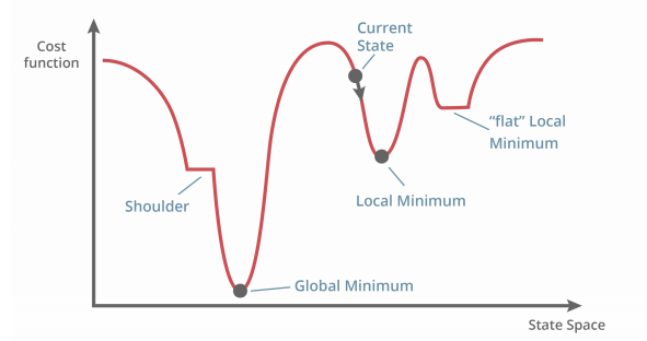
Gradient Descent
We can find a low error by taking the steepest downhill direction. We shouldn’t use step function as it is discontinuous - use other activation functions.
We can then adjust the weights and take this direction: $w\leftarrow w - \eta \frac{\delta E}{\delta w}$
Where: $\frac{\delta E}{\delta z} = \sum(z-t)$
And: $\frac{\delta z}{\delta s}$:
- For sigmoid: $z(s)=\sigma,\space z’(s)=z(1-z)$
- For tanh: $z(s)=tanh(s),\space z’(s)=1-z^2$
You find a local minimum (or global minimum) when the error $\frac{\delta E}{\delta z} = 0.$
Backpropogation
- Do a forward pass - with weights, output and calculte the error
- Backpropogation - do partial derivatives starting from the output back to the input, and multiply all together to obtain the new weights.
- This is efficient as you go backwards and you can reuse derivatives for other units.
Problems with Backprop
- Overfitting: when the training set error continues to reduce, but test set error starts to increase or stall
- Limit the number of hidden nodes or connections
- Limit the training time
- Weight decay - limit the growth/size of the weights - if the weights sharply increase in magnitude, NN is probably overfitting - large weights mean the output is jagged.
- Inputs/outputs should be re-scaled to be in the range 0 to 1 or -1 to 1
- When doing a forward pass, weights get multiplied by input, so the network emphasises inputs of larger magnitude
- Rescaling encourages inputs to be treated with equal importance
- Missing values should be replaced with mean values
- Weights should be initialised to very small random variables
- If weights are the same, they will all have the same error and model will not learn
- Should be set to around 0 so that weights do not need to change significantly (if very positive initial weight but should be a negative weight)
- Weights are dependent on the magnitude of the inputs (so, rescale/normalise the data)
- Training rate needs to be adjustd
- Too low and training will be very slow
- Too high and it may become unstable or skip minimums
Improvements to Backprop
- Online learning (stochastic gradient descent)
- In ‘vanilla’ gradient descent, we have $w\leftarrow w - \eta \frac{\delta E}{\delta w}$. $\delta E$ still has the sum of differences for all samples ($\frac{\delta E}{\delta z} = \sum(z-t)$). That is a lot of samples.
- Instead, we use the error of the latest training sample - $\frac{\delta E}{\delta z} = (z-t)$. Using the cost gradient of one sample instead of the sum of all.
- Weights are updated after each training item using differentials generated by that item - not the cost and gradient over the full training set.
- Batch learning
- Instead of using one sample (or all samples), aggregate many samples into ‘minibatches’ and update weights only after that batch is collected.
Applications of 2 Layer NNs
- Medical diagnosis
- Attributes: glucose concentration, blood pressure, skin fold thickness
- Autonomous driving, game playing
- ALVINN: Autonomous Land Vehicle In a Neural Network, with camera and later with sonar range finder
- Sonar with 8 x 32 input, 29 hidden units, 45 output
- ALVINN: Autonomous Land Vehicle In a Neural Network, with camera and later with sonar range finder
- Handwriting recognition
- Financial prediction
Resources
- http://colah.github.io/posts/2015-08-Backprop/ - The maths and reason behind backpropogation
- https://towardsdatascience.com/difference-between-batch-gradient-descent-and-stochastic-gradient-descent-1187f1291aa1+- How stochastic gradient descent works