Autoencoders
Autoencoders
- Unsupervised pretraining: pretrain using unsupervised method to get initial weights, then refine using backpropogation (then it becomes supervised)
- Better than backprop
- Encoder computes $z=f(x)$, decoder computes $g(f(x))$, we want to minimise the distance between z and g(f(x)):
$E = L(x, g(f(x)))$
Autoencoder Networks
- Input to bottleneck hidden layer = encoding
- Hidden to output layer = decoding
- After autoencoder is trained, decoder part is removed and replaced with, for example, a classification layer
- Greedy Layerwise Pretraining: alternative to RBM - hidden layer is trained to reconstruct the input. First layer (encoder) becomes first layer of deep network
Regularized Autoencoders
- Trivial identity: Often hidden nodes exceeds input nodes, might overfit (but free parameters might be less)
- Usually don’t pool as you lose information when decoding/reconstructing
- There is a risk that autoencoder reproduces the identity function - reproduce the input exactly, we want a new image
- Avoid by having very low number of weights/hidden nodes
- Or, introduce some form of regularisation - penalty to force weights to be restricted
Sparse autoencoders
- Add a penalty term based on the hidden unit activation - recall weight decay
- Instead of resizing weights, resize the hidden unit activations
$E = L(x, g(f(x))) + \lambda \sum_i|h_i|$
- This is L1 regularisation - absolute value rather than square - encourages some hidden units to go to 0, hence why it’s ‘sparse’ - features are present or absent
Contractive autoencoders
- Take derivative of hidden units and use L2 norm
$E = L(x, g(f(x))) + \lambda \sum_i||\triangledown_x h_i||^2$
- Forced to learn hidden features that don’t change much - small change in input is mapped to a very close point in the HU space
Denoising autoencoders
Add noise to inputs, train to recover original input
repeat:
    sample a training item x(i)
    generate a corrupted version x˜ of x(i)
    train to reduce E = L(x(i),g(f(x˜)))
end
Cost Functions and Probability
- Cost function can be seen as defining a probability distribution over the outputs - we train to maximise the log of the probability of the target values
- squared error assumes underlying Gaussian distribution, mean is the output of the network
- cross entropy assumes Bernoulli distribution, probability is the output of the network
- softmax assumes Boltzmann distribution
Stochastic Encoders and Decoders
- Decoder is a conditional proability distribution $p_\theta(x|z)$ of output x
- Encoder is a conditional proability distribution $q_\theta(z|x)$ of values z
- This is what we saw in RBM
Generative Models
- We want to make new images of bedrooms
- Explicit (Variational Autoencoders) or implicit (GANs)
Variational Autoencoders
- Instead of producing a single z, we want to produce a probability distribution with mean and sd - we train system to maximise:
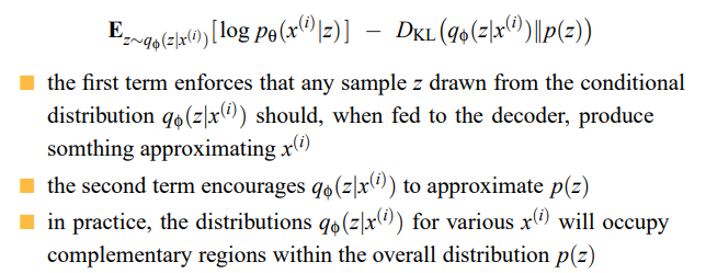
- First term is the probability of output being similar to the input
- Second term is the KL divergence
- Tension between both terms - KL divergence wants to stretch out the points to be the standard normal distribution, but in practice it will stretch certain dimensions out