Boltzmann Machines
Boltzmann Machines
- Motivation: Retrieve something from memory when presented only part of it.
- E.g. when given a set of images that are corrupted, reconstruct the original image
Hopfield Network
- Energy function is a cost function - local minima of energy function corresponds to the stored items
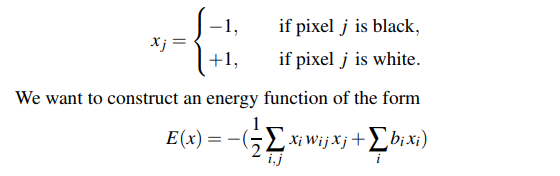
- For black and white images with $d$ pixels, where each image has a configuration $x = {x_j}_{1 \leq j \leq d}$ with:
- If we have p images, we have p local minima for E(x).
- Make $w_{ij}$ be positive if two pixels tend to have the same colour, $w_{ij}$ is negative if they are opposite colours.
- The 1/2 comes from assuming $w_{ij} = w_{ji}$ for all ij
- Weights for Hopfield networks are discrete - only -1 or +1
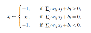
- To generate an image, we start with an initial state x and flip $x_i$ and try and reach a lower energy state. If we factor out $x_i$ from our E(x) expression, to reduce E(x) we change it to be:
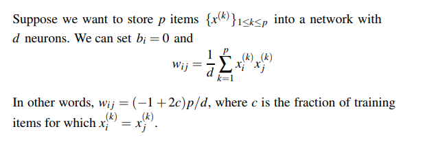
- Hebbian learning: update the weights according to the formula:
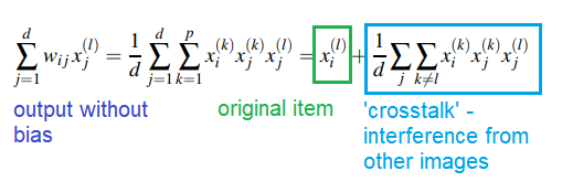
- For any image x:
- Reliably stored if $p/d < 0.138$, p the number of patterns and d the number of neurons in network
Generative Models
- What if we want to generate new items, not just store and retrieve past items? Generative model
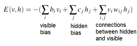
Boltzmann Machine
- Differences to Hopfield
- Energy function is the same
- Neurons $x_i$ are between 0 and 1, not -1/+1 (break inverted colour symmetry) - think of them as features
- Generate new states rather than retrieving stored state
- Update is not deterministic but stochastic
$p(x) = \frac{e^{-E(x)/T}}{Z}$
- E(x) is energy function, T is temperature, Z is partition function
- Similar to softmax but you want low energy = larger probability
- Gibbs Sampling: Have an image x, only change one pixel at a time - if changed, find energy change. Then, we can calculate conditional probability of $x_i$ taking the value 1 or 0

- Similar to Hopfield but there is randomness to updates.
- Boltzmann - we could have a change that moves the image to a higher energy state
- If repeated, eventually obtain a sample from Boltzmann distribution
- $T\rightarrow \infty,\space p(x_i\rightarrow1)=1/2$
- $T\rightarrow 0,\space p(x_i\rightarrow1)=0$ - behaviour becomes similar to Hopfield - energy never increases
- Temperature T is usually fixed at 1
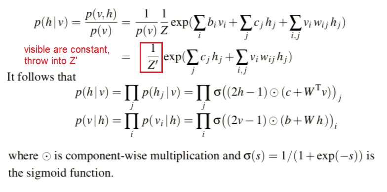
Restricted Boltzmann Machine
- Original Boltzmann - everything connected to everything - every pixel connected to each other one.
- RBM - introduce hidden units in addition to the visible pixel units
- No vis-to-vis or hidden-to-hidden connections
- Update becomes much faster - values for visible nodes fixed, change hidden nodes, and then vice versa
- Inputs are binary vectors
- Train to maximise expected log probability of the data
- Alternating Gibbs Sampling: Choose v0 randomly, sample h0 from p(h|v0), sample v1 from p(v|h0), etc. This is called ‘dreaming’
Training RBM
- Contrastive Divergence: Train by comparing real and fake images, prioritise the real ones
- Quick Contrastive Divergence: Start with real digit, generate hidden units, generate the false (reconstructed) digit and train using those as positive and negative samples respectively
- Not mathematically rigourous but good enough
Deep Boltzmann Machine
- Same approach but apply iteratively to multi-layer network
- Weights from input first layer trained first, then keep those fixed and train to second layer
Greedy Layerwise Pretraining
- Pair of layers trained as RBM, those values used as initial weights and biases for a feedforward NN, train using backprop and use for another task
https://www.doc.ic.ac.uk/~sd4215/hopfield.html